statistical inference
It Was Built for Batches
The hypothesis test taught in every introductory course is two rival frameworks spliced together by textbook writers after their authors stopped negotiating. The seam is visible in ordinary use, and the thing it hides is who holds each error.
- You are seeing
-
- A cutoff is described as a decision rule and nobody can state the alternative it was set against
- A threshold inherited from a previous system is defended on the grounds that it is standard
- The rate of wrongly admitted cases is tracked and the rate of wrongly rejected ones is not
- A score computed after the data is reported in the vocabulary of a pre-committed test
- Two desks disagree about a screen and neither can name which error the other is holding
- The mechanism
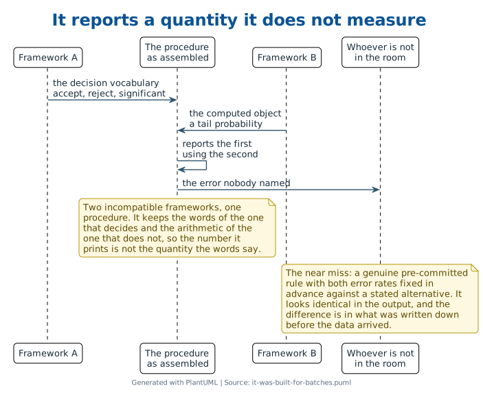
- A procedure assembled from two incompatible frameworks keeps the decision vocabulary of one and the computed object of the other, so it reports quantities it does not measure and the error nobody named goes to whoever is not in the room.
- The older apparatus
- Statistics, which conducted the disagreement in public under both men's names for twenty-seven years, and whose own histories record the splice as a splice rather than as a method.
- The false friend
- A genuine pre-committed decision rule with both error rates fixed in advance against a stated alternative. It looks identical in the output and is a different object, and the difference is whether anything was fixed before the data arrived.
- The discriminating test
- Ask what the alternative hypothesis is and what the rate of missing it has been. If the alternative cannot be named, the decision language is borrowed and the procedure is an evidence measure being read as a rule.
- On your own data
- For every threshold in production, record when it was set, against what alternative, and which desk absorbs each of the two error types. Count how many can populate all three fields.
Ronald Fisher published Statistical Methods for Research Workers in 1925, and it introduced significance testing in the form still practised: compute a p-value against a single null hypothesis, and treat 0.05 as a threshold worth a second look. Fisher described the number as convenient. He did not describe it as sacred.
His framework has no alternative hypothesis. It has no Type II error. It has no decision rule at all.
The p-value is evidence to weigh, computed after the data have been seen, with the researcher left to judge what worth investigating means in the case at hand.
Neyman and Pearson built the other thing #
Jerzy Neyman began working with Egon Pearson in 1927, looking for a general principle from which Gosset’s tests could be derived. What the pair produced between 1928 and 1933 was not a refinement.
Two hypotheses, a null and a specific alternative. A Type I rate and a Type II rate, both fixed before the data are collected. An outcome that is a mechanical accept or reject rather than a summary of evidence.
Their 1933 paper to the Royal Society proved that at a fixed error rate, testing one simple hypothesis against another, the likelihood-ratio test is the most powerful available. That is a real theorem and it is still true.
It is also a theorem about a situation nobody in a laboratory is in.
The dispute ran for twenty-seven years #
Fisher’s objection was not that the mathematics was wrong. It was that the framework had been built for industrial acceptance sampling — deciding whether to take delivery of a batch of manufactured goods — and did not describe research, where the working hypotheses are themselves revised as evidence accumulates.
Neyman held that Fisher’s fiducial inference was logically incoherent, and it is largely abandoned now.
That attempt is the part usually skipped, and it is the most telling thing in the episode. Fiducial inference was a route to a probability statement about a parameter without adopting a prior. The founder of the field tried to produce the quantity every user of a test actually wants — some probability attaching to the hypothesis itself — and could not get there without machinery he did not want to take on.
The two clashed bitterly and the question of which framework describes inference was never settled. The dispute ended in 1962, when Fisher died.
Neither man endorsed a merger of the two systems while he was alive to object.
The merger was performed by third parties #
From around 1940, introductory textbook writers combined them.
What is taught is Fisher’s single-null p-value, computed after the data are seen, reported in Neyman–Pearson’s decision vocabulary and surrounded by their mathematical apparatus. A researcher writing p = 0.03, therefore reject H₀ at α = 0.05 is running one framework’s language over the other’s object.
The seam is visible in ordinary use, and nobody maintains it, because the procedure has no author to maintain it.
The borrowed half is the vocabulary. Alpha, beta and power are defined only against a specific alternative hypothesis, and Fisher’s procedure does not have one. The terms describe quantities the computation does not produce.
Which gives the first test, and it is cheap. Ask what the alternative is. Where nobody can name it, the decision language came from somewhere else.
The same weld holds many screens #
A model produces a score after seeing the data. A policy consumes the score at a fixed cutoff and returns an accept or a reject.
The language around it is pre-committed — positions below the line are declined, applications below the line are refused — and the object underneath is an evidence measure with no alternative hypothesis attached and no measured rate of missing one.
Most cutoffs in use acquired their number the way 0.05 did. Somebody found it convenient, it was inherited, and the convenience became a boundary. That is not a criticism of the number. Fisher’s was fine too, for what he was doing with it.
A threshold that arrived with a vendor system, survived two migrations, and is now defended on the grounds that it is standard has a provenance rather than a justification, and the two get recorded in the same field.
The question is what is being claimed by putting decision language around it.
Acceptance sampling had two parties #
Fisher’s objection names the setting the other framework does fit, and it is worth taking literally rather than as a jibe.
A batch inspection has a producer and a buyer. The producer absorbs the cost of a good batch wrongly rejected. The buyer absorbs the cost of a bad batch wrongly accepted. The two error rates are the terms of a negotiation between two parties who each hold one of them and know which one they are holding.
That is what makes the pre-commitment real. The numbers are contractual before they are statistical.
A laboratory has no counterparty, which is Fisher’s complaint restated.
An institution has one, and it is internal. A screen that rejects a good position costs the desk that would have held it. A screen that admits a bad one costs the people who carry the loss. The two errors land in different places and only one of them reliably generates a report, because a position that was never taken does not produce an incident.
So the unmeasured rate is not unmeasured by accident. It is the one whose owner was not in the room when the cutoff was set.
Fisher and Neyman argued for twenty-seven years and neither of them won. The textbooks resolved it by printing both and letting the seam show.
A firm that cannot name its alternative hypothesis has resolved it the same way, and the desk holding the error nobody counts is the one that did not get a say in the number.
Questions
Who invented the hypothesis test?
Nobody, and that is the useful fact about it. Ronald Fisher built significance testing in the 1920s: one null hypothesis, a p-value computed after the data are seen, and a 0.05 threshold he described as convenient rather than sacred. Jerzy Neyman and Egon Pearson built a different thing between 1928 and 1933: two hypotheses, both error rates fixed before collection, and a mechanical accept-or-reject outcome. Textbook authors combined them from about 1940. Neither originator endorsed the combination.
Why does the standard testing procedure feel internally inconsistent?
Because it is. The phrase reject the null at α = 0.05 runs Neyman–Pearson decision vocabulary over Fisher's post hoc evidence measure, and the two were never designed to compose. Fisher's framework has no alternative hypothesis and no Type II error, so the α and β and power language borrowed from the other side describes quantities his procedure does not produce. Readers who push on the seam are finding a real one.
What was Fisher's actual objection to the Neyman–Pearson framework?
That it was built for industrial acceptance sampling — deciding whether to take delivery of a batch of manufactured goods — and did not describe a research setting, where the working hypotheses are revised as evidence accumulates. He was describing a fit between a method and a situation rather than an error in the mathematics. The Neyman–Pearson lemma is a genuine 1933 optimality theorem and remains one.
How can you tell whether a threshold in use is a real decision rule?
Ask when it was set and against what. A pre-committed rule has an alternative it was set against and a stated rate of missing that alternative, both fixed before the data arrived. A cutoff that acquired its number from a previous system, or from what looked reasonable once the distribution was visible, is an evidence measure wearing decision language. The two produce identical output and are different claims about what has been controlled. Fisher's own 0.05 was the second kind, and he said so, describing it as convenient rather than sacred.
Why does acceptance sampling get away with pre-committed error rates?
Because both errors have owners who are negotiating with each other. The producer absorbs the cost of a good batch rejected; the buyer absorbs the cost of a bad batch accepted. The two rates are contractual terms between parties who each hold one of them and know which. Where a screen sits inside one institution, the two errors still land in different places, and usually only one of them generates an incident report.